
Introduction
Machine learning models are designed to learn patterns from data and make accurate predictions on new, unseen information. However, one of the most common challenges beginners encounter is balancing model complexity and performance. This is where the concepts of overfitting vs underfitting in machine learning become critically important.
Think about the Goldilocks principle: not too simple, not too complex — but just right. Machine learning models follow a similar idea. If a model is too simple, it fails to learn important patterns from the dataset. If it is too complex, it memorizes the training data instead of learning the underlying patterns.
These two problems are known as:
- Underfitting – when a model is too simple to capture the structure of the data.
- Overfitting – when a model learns the noise in the data instead of the real patterns.
Understanding the difference between overfitting vs underfitting in machine learning is essential if you want to build models that perform well on real-world data.
Many beginner machine learning projects fail not because the algorithms are wrong, but because these two issues are ignored.
In this beginner-friendly Python guide, you will learn:
- What overfitting and underfitting mean in machine learning
- Why model generalization matters
- How to detect these problems using training and testing performance
- How to demonstrate overfitting and underfitting using Python and scikit-learn
- Practical solutions to prevent these problems
By the end of this guide, you will clearly understand how to recognize and fix overfitting and underfitting in machine learning models using Python.
If you are new to machine learning pipelines, you may want to first understand the Machine Learning Workflow in Python before diving deeper into model performance issues.
Prerequisites
Before continuing, you should have basic knowledge of:
- Python programming
- NumPy and Pandas
- Basic machine learning concepts
- The scikit-learn library
If you are new to machine learning workflows, you may want to read our guide on Machine Learning Workflow in Python before continuing.
Understanding the Basics
Before we dive into Python implementations, it is important to understand the fundamental concepts behind overfitting vs underfitting in machine learning.
What is Model Generalization?
In machine learning, the ultimate goal is not simply to perform well on training data. Instead, the goal is to create models that generalize well to new data.
Machine learning models are usually evaluated using a training dataset and a testing dataset created using techniques like Train Test Split in Python for Machine Learning.
Generalization refers to a model’s ability to make accurate predictions on unseen data.
When a machine learning model is trained, the dataset is typically divided into two parts:
- Training dataset – used to train the model
- Testing dataset – used to evaluate the model’s performance
This process is commonly done using train-test splitting.
If you want a detailed explanation of this process, check our guide on Train Test Split in Python for Machine Learning.
A well-performing model should have:
- Low training error
- Low testing error
However, when models become too simple or too complex, problems appear.
These problems are known as:
- Underfitting
- Overfitting
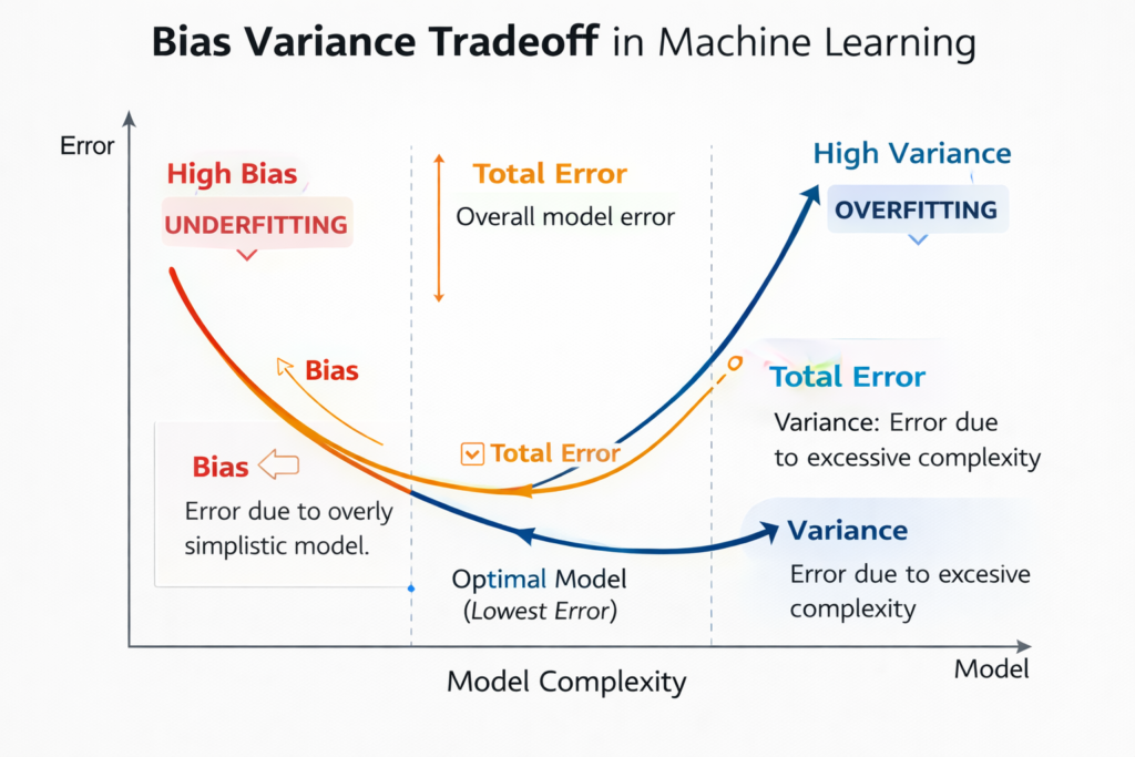
The Bias-Variance Tradeoff
To fully understand overfitting vs underfitting in machine learning, we must understand the bias-variance tradeoff.
The relationship between model complexity, bias, and variance is known as the bias-variance tradeoff explained in machine learning theory.
This concept explains why machine learning models sometimes fail to generalize.
Bias
Bias represents the error introduced by overly simple assumptions in a model.
Models with high bias:
- Are too simple
- Fail to capture important patterns
- Lead to underfitting
Variance
Variance represents the model’s sensitivity to small fluctuations in the training data.
Models with high variance:
- Learn the training data too closely
- Capture noise instead of patterns
- Lead to overfitting
The Tradeoff
The challenge in machine learning is finding the right balance:
| Model Type | Bias | Variance |
|---|---|---|
| Underfitting | High | Low |
| Good Fit | Balanced | Balanced |
| Overfitting | Low | High |
The best machine learning models achieve the right balance between bias and variance.
Underfitting in Machine Learning
Let’s first understand underfitting, one side of the overfitting vs underfitting in machine learning problem.
What is Underfitting?
Underfitting occurs when a machine learning model is too simple to learn the underlying structure of the data.
This means the model fails to capture meaningful patterns.
As a result, the model performs poorly on both training data and testing data.
In simple terms:
The model has not learned enough from the data.
Characteristics of Underfitting
Underfitting models usually have the following characteristics:
- High training error
- High testing error
- Poor predictive performance
- High bias
- Low variance
This happens when the model is too simple for the complexity of the dataset.
Example of Underfitting
Imagine you are trying to predict house prices using only one feature, such as the number of rooms.
But the real factors affecting house prices include:
- Location
- Size
- Neighborhood quality
- Distance from city center
- Market trends
Using a very simple model in this case would result in underfitting because the model ignores important information.
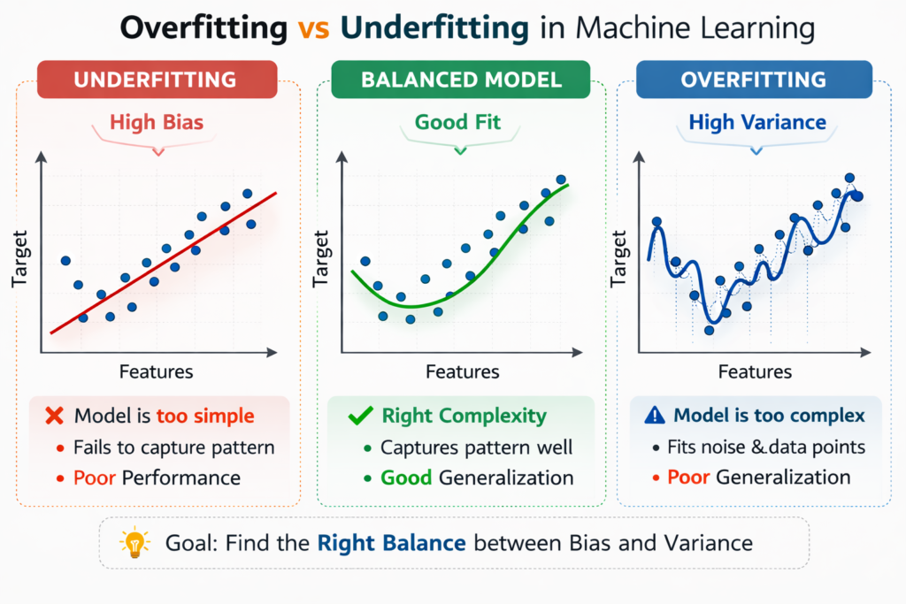
Visual Analogy
A common way to understand underfitting is by imagining a straight line trying to fit curved data.
If the dataset follows a curved pattern but the model only fits a straight line, the model will miss important trends.
This leads to high prediction errors.
Overfitting in Machine Learning
Now let’s examine the opposite problem in overfitting vs underfitting in machine learning.
What is Overfitting?
Overfitting occurs when a machine learning model learns the training data too well, including noise and random fluctuations.
Instead of learning general patterns, the model memorizes the training dataset.
As a result:
- Training performance becomes extremely good
- Testing performance becomes poor
This means the model cannot generalize to new data.
Characteristics of Overfitting
Overfitting models usually show the following behavior:
- Very low training error
- High testing error
- High variance
- Poor generalization
- Model complexity is too high
Example of Overfitting
Imagine a student preparing for an exam by memorizing every practice question.
If the real exam questions are different, the student may struggle because they memorized answers instead of understanding the concepts.
Machine learning models behave in the same way.
When models memorize training data, they fail on new data.
Visual Analogy
In a graph, overfitting appears as a very complex curve passing through almost every training point.
While the curve perfectly matches the training dataset, it becomes extremely sensitive to noise.
This results in poor predictions on unseen data.
Comparing Overfitting vs Underfitting in Machine Learning
Understanding the differences between these two problems helps you diagnose machine learning models quickly.
| Problem | Training Accuracy | Testing Accuracy | Cause |
|---|---|---|---|
| Underfitting | Low | Low | Model too simple |
| Good Fit | High | High | Balanced complexity |
| Overfitting | Very High | Low | Model too complex |
The goal of machine learning is always to achieve the good fit scenario.
Python Setup and Dataset Preparation
Now that we understand the theory behind overfitting vs underfitting in machine learning, let’s demonstrate these problems using Python.
The examples in this tutorial use the scikit-learn official documentation to implement machine learning models in Python.
We will create a simple dataset and train different models to observe how underfitting and overfitting occur.
Required Libraries
First, import the necessary Python libraries.
import numpy as np
import pandas as pd
import matplotlib.pyplot as plt
import seaborn as sns

from sklearn.model_selection import train_test_split
from sklearn.preprocessing import PolynomialFeatures
from sklearn.linear_model import LinearRegression
from sklearn.metrics import mean_squared_error
These libraries allow us to:
- Generate synthetic datasets
- Train machine learning models
- Visualize results
- Evaluate model performance
Creating a Synthetic Dataset
To clearly demonstrate overfitting vs underfitting in machine learning, we will create a nonlinear dataset.
# Generate nonlinear data
np.random.seed(42)

X = np.sort(np.random.rand(100,1) * 10, axis=0)
y = np.sin(X).ravel() + np.random.normal(0,0.1,X.shape[0])
This dataset follows a sine curve pattern, which is useful for demonstrating model complexity.
Train-Test Split
Next, we divide the dataset into training and testing sets.
X_train, X_test, y_train, y_test = train_test_split(
    X, y, test_size=0.3, random_state=42
)
Here:
- 70% of the data is used for training
- 30% is used for testing
This allows us to evaluate how well the model generalizes to unseen data.
Demonstrating Underfitting in Python
Let’s begin by creating a very simple model.
This will demonstrate underfitting.
Linear Model (Degree 1)
model_under = LinearRegression()

model_under.fit(X_train, y_train)

y_train_pred = model_under.predict(X_train)
y_test_pred = model_under.predict(X_test)

train_error = mean_squared_error(y_train, y_train_pred)
test_error = mean_squared_error(y_test, y_test_pred)

print("Training Error:", train_error)
print("Testing Error:", test_error)
Because the data follows a nonlinear sine pattern, a simple linear regression model will struggle to capture the relationship.
As a result:
- Training error will be high
- Testing error will also be high
This is a classic example of underfitting in machine learning.
Visualizing the Underfitting Model
You can visualize the results using Matplotlib.
plt.scatter(X, y)
plt.plot(X, model_under.predict(X), color='red')
plt.title("Underfitting Example")
plt.show()
The straight red line fails to follow the curve of the dataset.
This confirms that the model is too simple to learn the pattern.
Demonstrating a Good Fit Model
After seeing an underfitting model, the next step is to create a model that properly captures the structure of the dataset.
The dataset we generated earlier follows a sine curve pattern. A linear model cannot capture that curve, but a polynomial regression model can.
Polynomial regression increases model complexity by adding polynomial features.Polynomial models allow algorithms to capture nonlinear relationships, which is explained in detail in polynomial regression in machine learning.
Polynomial Model (Degree 4)
Let’s build a polynomial regression model that is complex enough to capture the curve but not too complex to cause overfitting.
from sklearn.preprocessing import PolynomialFeatures
from sklearn.linear_model import LinearRegression

# Create polynomial features
poly_features = PolynomialFeatures(degree=4, include_bias=False)

X_poly_train = poly_features.fit_transform(X_train)
X_poly_test = poly_features.transform(X_test)

# Train model
model_good = LinearRegression()
model_good.fit(X_poly_train, y_train)

# Predictions
y_train_pred = model_good.predict(X_poly_train)
y_test_pred = model_good.predict(X_poly_test)

# Calculate errors
train_error = mean_squared_error(y_train, y_train_pred)
test_error = mean_squared_error(y_test, y_test_pred)

print("Training Error:", train_error)
print("Testing Error:", test_error)
In this case, the model is complex enough to capture the sine curve pattern but not too complex to memorize noise.
You will usually see:
- Low training error
- Low testing error
This indicates a well-balanced model.
Visualization of a Good Fit
To understand this better, let’s visualize the model.
plt.scatter(X, y)

X_range = np.linspace(0,10,100).reshape(-1,1)
X_range_poly = poly_features.transform(X_range)

plt.plot(X_range, model_good.predict(X_range_poly), color='green')

plt.title("Good Fit Model")
plt.show()
The curve now follows the structure of the dataset smoothly.
This demonstrates the ideal scenario in machine learning — the model captures patterns but ignores random noise.
This is the goal when solving overfitting vs underfitting in machine learning problems.
Demonstrating Overfitting in Python
Now let’s move to the opposite extreme.
Instead of making the model slightly more complex, we will make it extremely complex.
This will produce overfitting.
High-Degree Polynomial Model
We will create a polynomial model with degree 15.
poly_features = PolynomialFeatures(degree=15, include_bias=False)

X_poly_train = poly_features.fit_transform(X_train)
X_poly_test = poly_features.transform(X_test)

model_over = LinearRegression()
model_over.fit(X_poly_train, y_train)

y_train_pred = model_over.predict(X_poly_train)
y_test_pred = model_over.predict(X_poly_test)

train_error = mean_squared_error(y_train, y_train_pred)
test_error = mean_squared_error(y_test, y_test_pred)

print("Training Error:", train_error)
print("Testing Error:", test_error)
In most cases you will observe:
- Extremely low training error
- High testing error
The model has essentially memorized the training dataset.
Visualization of Overfitting
plt.scatter(X, y)

X_range = np.linspace(0,10,100).reshape(-1,1)
X_range_poly = poly_features.transform(X_range)

plt.plot(X_range, model_over.predict(X_range_poly), color='purple')

plt.title("Overfitting Example")
plt.show()
Instead of a smooth curve, the model produces a very wiggly line.
This line tries to pass through almost every training point.
While this looks impressive on training data, it performs poorly on new data.
This is the core problem in overfitting vs underfitting in machine learning.
Understanding Learning Curves
Learning curves are one of the most powerful tools for diagnosing machine learning models.
They show how model performance changes as the training dataset size increases.
Learning curves help identify:
- Underfitting
- Overfitting
- Balanced models
Creating Learning Curves in Python
We can use scikit-learn’s learning_curve function.
from sklearn.model_selection import learning_curve

train_sizes, train_scores, validation_scores = learning_curve(
    model_good,
    X,
    y,
    cv=5,
    scoring='neg_mean_squared_error',
    train_sizes=np.linspace(0.1,1.0,10)
)
This function evaluates model performance on different dataset sizes.
Plotting Learning Curves
train_scores_mean = -train_scores.mean(axis=1)
validation_scores_mean = -validation_scores.mean(axis=1)

plt.plot(train_sizes, train_scores_mean, label="Training Error")
plt.plot(train_sizes, validation_scores_mean, label="Validation Error")

plt.xlabel("Training Size")
plt.ylabel("Error")
plt.title("Learning Curve")
plt.legend()

plt.show()
This plot provides critical insights into overfitting vs underfitting in machine learning.
Interpreting Learning Curves
Let’s look at how learning curves help diagnose problems.
Learning Curve for Underfitting
In an underfitting model:
- Training error is high
- Validation error is also high
- Both curves converge
This means the model is too simple to learn the data patterns.
Learning Curve for Overfitting
In an overfitting model:
- Training error is extremely low
- Validation error is much higher
- Large gap between curves
This indicates the model is memorizing training data instead of generalizing.
Learning Curve for Good Fit
In a well-trained model:
- Training error is low
- Validation error is also low
- Curves converge closely
This indicates a balanced model.
Detecting Overfitting and Underfitting
Understanding theory is useful, but in real machine learning projects we must diagnose these problems quickly.
Here are the most common signs.
Key Signs in Practice
| Symptom | Training Accuracy | Validation Accuracy | Diagnosis |
|---|---|---|---|
| Both low | Low | Low | Underfitting |
| Both high | High | High | Good Fit |
| Large gap | High | Low | Overfitting |
This simple table is widely used by machine learning engineers.
It helps quickly identify overfitting vs underfitting in machine learning models.
Using Cross-Validation
Cross-validation is another powerful technique for detecting model issues.
Instead of using a single train-test split, the dataset is divided into multiple folds.
The model is trained and evaluated several times.
Cross-Validation Example in Python
from sklearn.model_selection import cross_val_score

scores = cross_val_score(
    model_good,
    X,
    y,
    cv=5,
    scoring='neg_mean_squared_error'
)

print("Cross Validation Scores:", scores)
print("Average Score:", scores.mean())
Cross-validation provides:
- More reliable model evaluation
- Reduced risk of misleading results
- Better detection of overfitting
Because of these benefits, cross-validation is a standard practice in machine learning.
Why Beginners Often Face Overfitting
Many beginner machine learning projects suffer from overfitting.
Common reasons include:
- Using very complex models
- Training on small datasets
- Ignoring regularization
- Not using cross-validation
- Testing the model on the same data used for training
Understanding overfitting vs underfitting in machine learning helps prevent these mistakes.
Why Underfitting Happens
Underfitting usually happens when models are too simple.
Common causes include:
- Using linear models for nonlinear data
- Removing too many features
- Excessive regularization
- Insufficient training time
While underfitting is easier to fix than overfitting, it still leads to poor predictions.
Solutions for Underfitting
Underfitting happens when the model is too simple to capture the structure of the data.
Fortunately, underfitting is usually easier to fix than overfitting.
Below are the most effective solutions.
1. Increase Model Complexity
The most common reason for underfitting is that the model is too simple.
For example:
- Linear regression may not capture nonlinear relationships.
- Decision trees with very small depth may miss important patterns.
Increasing model complexity can solve this problem.
Examples include:
- Using polynomial regression
- Increasing tree depth
- Using more advanced algorithms
2. Add More Features
Sometimes the model fails because the dataset lacks important information.
For example, predicting house prices using only one feature may cause underfitting.
Adding relevant features improves the model’s ability to learn patterns.
Examples of useful features:
- Location data
- Historical trends
- Derived features (feature engineering)
Feature engineering is a powerful tool in machine learning.
3. Reduce Regularization
Regularization techniques prevent overfitting by penalizing large model weights.
However, excessive regularization may make the model too simple.
If regularization strength is too high, the model may suffer from underfitting.
Reducing regularization strength can improve model performance.
4. Train the Model Longer
Some algorithms, especially neural networks, require longer training time.
Stopping the training process too early may prevent the model from learning useful patterns.
Increasing the number of training iterations can sometimes fix underfitting.
One effective way to reduce underfitting is through Feature Engineering in Python for Machine Learning, which helps models capture more meaningful patterns.
Solutions for Overfitting
Overfitting is more challenging because the model already performs well on training data but poorly on new data.
Below are the most effective solutions used in machine learning.
1. Use Cross-Validation
Cross-validation evaluates the model on multiple dataset splits.
This reduces the risk of misleading results caused by a single train-test split.
Cross-validation ensures that the model performs consistently across different subsets of data.
Example in Python:
from sklearn.model_selection import cross_val_score

scores = cross_val_score(
    model_good,
    X,
    y,
    cv=5,
    scoring='neg_mean_squared_error'
)

print("Average CV Score:", scores.mean())
Cross-validation is considered a standard practice in machine learning workflows.
2. Regularization Techniques
Regularization reduces model complexity by penalizing large coefficients.
Two common regularization techniques are:
- Ridge Regression
- Lasso Regression
These methods are widely used to control overfitting in machine learning models.
Regularization methods such as Ridge and Lasso regression explained help control model complexity and reduce overfitting.
Ridge Regression Example
Ridge regression adds a penalty to large model weights.
This helps prevent models from becoming overly complex.
from sklearn.linear_model import Ridge

ridge_model = Ridge(alpha=1.0)

ridge_model.fit(X_train, y_train)

predictions = ridge_model.predict(X_test)

print("Ridge Model Predictions:", predictions[:5])
The parameter alpha controls regularization strength.
Higher alpha values increase regularization.
Lasso Regression Example
Lasso regression performs regularization and feature selection simultaneously.
from sklearn.linear_model import Lasso

lasso_model = Lasso(alpha=0.1)

lasso_model.fit(X_train, y_train)

predictions = lasso_model.predict(X_test)

print("Lasso Predictions:", predictions[:5])
Lasso is particularly useful when dealing with high-dimensional datasets.
3. Collect More Training Data
One of the most effective ways to reduce overfitting is simply using more data.
With larger datasets:
- Models are less likely to memorize noise
- Patterns become easier to identify
- Variance decreases
In real-world machine learning projects, collecting more data is often the best solution.
4. Reduce Model Complexity
Another approach is to simplify the model.
Examples include:
- Reducing polynomial degree
- Limiting decision tree depth
- Using fewer features
Simpler models are less likely to memorize training data.
5. Data Augmentation
In some fields like computer vision, collecting data may be difficult.
In such cases, data augmentation can help.
Examples include:
- Rotating images
- Flipping images
- Adding noise
- Scaling images
These techniques increase dataset diversity and reduce overfitting.
6. Early Stopping
Early stopping is commonly used in deep learning.
During training, model performance on validation data is monitored.
Training stops when validation performance begins to degrade.
This prevents the model from learning noise in the dataset.
Real-World Example: California Housing Dataset
Now let’s apply these concepts to a real dataset.
We will use the California Housing dataset, which is available in scikit-learn.
Loading the Dataset
from sklearn.datasets import fetch_california_housing

data = fetch_california_housing()

X = data.data
y = data.target
This dataset contains features such as:
- Median income
- House age
- Average rooms
- Population
- Location coordinates
The target variable is the median house value.
Train-Test Split
from sklearn.model_selection import train_test_split

X_train, X_test, y_train, y_test = train_test_split(
    X, y, test_size=0.2, random_state=42
)
Training a Linear Regression Model
from sklearn.linear_model import LinearRegression

model = LinearRegression()

model.fit(X_train, y_train)

predictions = model.predict(X_test)
Evaluating Model Performance
from sklearn.metrics import mean_squared_error

mse = mean_squared_error(y_test, predictions)

print("Mean Squared Error:", mse)
This gives us a baseline model.
From here, we can experiment with:
- Regularization
- Feature engineering
- Model complexity
These techniques help solve overfitting vs underfitting in machine learning models.
Practical Tips for Machine Learning Projects
Below are some best practices used by professional data scientists.
Start with Simple Models
Always begin with simple algorithms like:
- Linear Regression
- Logistic Regression
- Decision Trees
These models help establish a baseline.
Once the baseline is understood, you can move to more complex algorithms.
Monitor Training and Validation Performance
Never rely only on training accuracy.
Always evaluate models on validation or testing datasets.
Large differences between training and validation performance often indicate overfitting.
Use Cross-Validation Regularly
Cross-validation reduces bias in model evaluation.
Most professional machine learning pipelines include cross-validation as a standard step.
Keep a Separate Test Dataset
The test dataset should only be used once at the final stage of evaluation.
Using the test dataset during training may lead to misleading results.
Quick Reference Guide
Here is a simple summary of overfitting vs underfitting in machine learning.
| Problem | Cause | Solution |
|---|---|---|
| Underfitting | Model too simple | Increase complexity |
| Overfitting | Model too complex | Add regularization |
| Overfitting | Small dataset | Collect more data |
| Underfitting | Missing features | Feature engineering |
This table is useful when diagnosing machine learning models.
Key Takeaways
Let’s summarize the most important lessons from this guide.
- Overfitting vs underfitting in machine learning describes two common model performance problems.
- Underfitting occurs when the model is too simple to capture data patterns.
- Overfitting occurs when the model memorizes training data instead of learning patterns.
- The goal is to find the right balance between bias and variance.
- Techniques such as cross-validation, regularization, and feature engineering help improve model performance.
Mastering these concepts is essential for building reliable machine learning systems.
Practice Exercises
To strengthen your understanding, try the following exercises.
Exercise 1
Modify the polynomial degree in the earlier example.
Observe how the training and testing errors change.
Try values like:
- Degree 2
- Degree 5
- Degree 10
Exercise 2
Experiment with Ridge Regression using different alpha values.
Try:
- alpha = 0.1
- alpha = 1
- alpha = 10
Observe how model performance changes.
Exercise 3
Create your own synthetic dataset using NumPy.
Try to identify:
- Underfitting
- Good fit
- Overfitting
Additional Resources
To deepen your understanding of overfitting vs underfitting in machine learning, consider the following resources.
Recommended books:
- Introduction to Statistical Learning
- Elements of Statistical Learning
Useful documentation:
- scikit-learn official documentation
- Python data science tutorials
These resources provide deeper theoretical explanations and practical examples.
Final Thoughts
Understanding overfitting vs underfitting in machine learning is one of the most important steps for anyone starting a machine learning journey.
Most beginners focus heavily on algorithms, but the real success of machine learning projects often depends on how well models generalize to unseen data.
By learning how to detect and fix these issues using Python, you are already developing the mindset of a professional machine learning engineer.
As you build more projects, always remember the key principle:
The goal of machine learning is not perfect training performance — it is reliable real-world predictions.
Once you understand model evaluation concepts like overfitting and underfitting, you can apply them to real projects such as Build an AI Text Analyzer with Python.
FAQ – Overfitting vs Underfitting in Machine Learning
What is overfitting vs underfitting in machine learning?
Underfitting occurs when a model is too simple and cannot learn the patterns in the data.
Overfitting occurs when a model is too complex and memorizes the training data instead of learning general patterns.
How can you detect overfitting and underfitting?
You can detect these problems by comparing training and testing performance.
High training error + high testing error → Underfitting
Low training error + high testing error → Overfitting
What causes overfitting in machine learning?
Overfitting usually happens due to:
Very complex models
Small datasets
Too many features
Lack of regularization
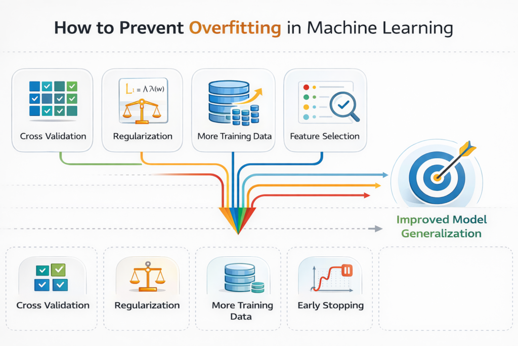
How can overfitting be prevented?
Common ways to prevent overfitting include:
Using cross-validation
Applying regularization (Ridge or Lasso)
Reducing model complexity
Collecting more data
What causes underfitting in machine learning?
Underfitting happens when the model is too simple or does not have enough features to learn the data patterns.
Why is train-test split important?
Train-test split allows you to evaluate model performance on unseen data, helping detect overfitting and underfitting.

