Introduction: Why Text Classification Matters in 2026
Text classification in Python is one of the most important techniques in modern Natural Language Processing (NLP). It allows developers to automatically categorize large volumes of text such as customer support messages, product reviews, emails, and social media posts.
As the amount of digital text continues to grow, businesses increasingly rely on machine learning models to analyze and organize this data efficiently.
We are living through an unprecedented explosion of text data. Research estimates that roughly 80% of enterprise data is now unstructured — emails, support tickets, reviews, social media posts, legal documents, and more. Buried inside this torrent of words is signal: customer frustration, product feedback, security threats, purchase intent. The challenge is extracting it at scale. That is exactly where text classification comes in.
What is Text Classification?
Text classification is the task of automatically assigning predefined categories to free-form text. If you’ve ever wondered how Gmail separates spam from real messages, how Spotify knows you’re asking for a “chill playlist” versus a “workout playlist,” or how your bank flags fraudulent transaction notes — you’ve already encountered text classifiers in the wild.
Common real-world forms include:
- Sentiment Analysis — is this review positive, negative, or neutral?
- Spam Detection — is this email junk?
- Intent Recognition — is the user trying to book a flight, cancel a subscription, or ask a question?
- Topic Labeling — does this article belong in Sports, Finance, or Technology?
- Support Ticket Routing — should this ticket go to Billing, Technical Support, or Returns?
Why Python?
Python has dominated the NLP landscape for years, and 2026 is no different. The ecosystem is simply unmatched. scikit-learn gives you battle-tested classical algorithms in a consistent API. spaCy handles industrial-strength linguistic preprocessing. And Hugging Face — with over 500,000 models on its Hub — has become the de-facto standard for state-of-the-art transformer-based NLP. You can go from idea to fine-tuned BERT model in under 50 lines of code.
What You’ll Build
🎯 The Project: Customer Support Ticket Classifier
By the end of this guide, you’ll have a working multi-class classifier that reads an incoming customer support message and predicts its category: Billing, Technical Issue, Shipping, or Account Management. We’ll build it twice — once the fast way with Logistic Regression, and once the powerful way with DistilBERT.
In this guide you will learn:• What text classification is
- How to preprocess text with spaCy
- How to build a TF-IDF + Logistic Regression classifier
- How to fine-tune DistilBERT
- How to evaluate NLP models correctly
02The 2026 Tech Stack
Before writing a single line of model code, let’s get oriented on our tools. The NLP ecosystem has matured significantly, and making the right choices upfront saves enormous refactoring time later.
Data Wrangling: Polars
If you’ve been writing import pandas as pd on autopilot, it’s time to reconsider. Polars is a lightning-fast DataFrame library written in Rust with a Python API. It uses lazy evaluation and Apache Arrow under the hood, making it 5–20× faster than Pandas on most text-heavy workloads. For 2026 projects, Polars is the recommended default for any dataset over a few thousand rows.
Core NLP: spaCy
spaCy is an industrial-strength NLP library designed for real-world pipelines, not academic toy examples. It ships with pretrained models for tokenization, part-of-speech tagging, named entity recognition, and dependency parsing across dozens of languages. Its pipeline architecture makes it trivially easy to batch-process millions of documents in parallel.
Modeling: Two Tiers
We’ll use a two-tier approach that mirrors real-world engineering practice. Start classical, upgrade only when necessary.
Tier 1 — Classic ML
scikit-learn
Naive Bayes, Logistic Regression, and SVM. Fast to train, easy to interpret, deployable anywhere. Often shockingly competitive with deep learning on clean data.
Machine learning model section.
Tier 2 — Deep Learning
Hugging Face Transformers
DistilBERT, RoBERTa, and friends. Contextual embeddings that understand nuance. The Trainer API makes fine-tuning accessible to everyone.
Environment Setup
Create a fresh virtual environment and install everything in one shot:
# Create and activate a virtual environment
python -m venv nlp-env
source nlp-env/bin/activate  # Windows: nlp-env\Scripts\activate

# Install all dependencies
pip install polars spacy scikit-learn transformers datasets \
            seaborn matplotlib torch --index-url https://download.pytorch.org/whl/cpu

# Download the spaCy English model
python -m spacy download en_core_web_sm
💡
PyTorch CPU vs GPU
For this tutorial, the CPU version of PyTorch is sufficient. If you have an NVIDIA GPU and want significantly faster fine-tuning, swap cpu for cu121 (for CUDA 12.1) in the install URL.
Types of Text Classification
Explain:
- Binary classification
- Multi-class classification
- Multi-label classification
Example:
Binary classification:
Spam vs Not SpamMulti-class classification:
Billing / Technical / ShippingMulti-label classification:
A message can belong to multiple categories
Before building a classifier, proper text cleaning is essential. Learn the full preprocessing workflow in our guide on text preprocessing in Python.
Step 1: Data Acquisition for Text Classification in Python and Exploration
Good models start with good data. Fortunately, the Hugging Face datasets library gives us instant, reproducible access to thousands of curated NLP datasets — no manual downloading or CSV wrangling required.
Loading Data
We’ll use the Banking77 dataset — a popular benchmark containing 13,000+ customer banking queries across 77 intent categories. We’ll simplify it to 5 broad categories to match our support ticket use case.
from datasets import load_dataset
import polars as pl

# Load the dataset directly from Hugging Face Hub
raw = load_dataset("banking77", split="train")

# Convert to a Polars DataFrame for fast manipulation
df = pl.DataFrame({
    "text": raw["text"],
    "label": raw["label"]
})

print(df.head(5))
print(f"Dataset shape: {df.shape}")
Exploratory Data Analysis (EDA)
Before building anything, you need to understand your data. Two questions matter most: Are the classes balanced? And what distinguishes one category from another?
import seaborn as sns
import matplotlib.pyplot as plt
from collections import Counter

# Plot class distribution
label_counts = df["label"].value_counts().sort("count", descending=True)

plt.figure(figsize=(12, 5))
sns.barplot(
    x=label_counts["label"].to_list(),
    y=label_counts["count"].to_list(),
    palette="viridis"
)
plt.title("Class Distribution in Banking77", fontsize=14)
plt.xticks(rotation=45, ha="right")
plt.tight_layout()
plt.show()
Look for class imbalance — if one category has 10× more samples than another, your model will be biased toward predicting it. Techniques like oversampling (SMOTE) or class-weight adjustments in scikit-learn can compensate.
Next, find the “top words” per category to get a feel for what makes each class distinctive. Spoiler: you’ll often find obvious signal words that make the task easier than expected — and also red herrings that could cause the model to overfit.
from sklearn.feature_extraction.text import CountVectorizer
def top_words_per_class(df, label_col, text_col, top_n=10):
for label in df[label_col].unique().to_list():
subset = df.filter(pl.col(label_col) == label)[text_col].to_list()
vec = CountVectorizer(stop_words="english", max_features=top_n)
vec.fit(subset)
words = list(vec.vocabulary_.keys())
print(f"Label {label}: {', '.join(words)}")
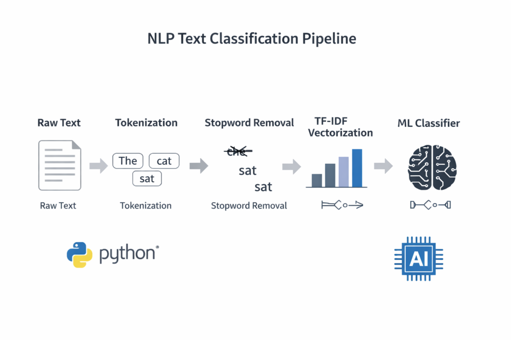
top_words_per_class(df, "label", "text")04Step 2: Modern Preprocessing — The “Clean” Phase
Raw text is messy. It contains typos, HTML artifacts, emoji, inconsistent casing, and filler words that add noise without adding meaning. Preprocessing is how we reduce this noise and help the model focus on what matters.
Tokenization & Lemmatization
Tokenization splits a sentence into individual units (tokens). Lemmatization reduces each token to its base dictionary form: “running” → “run”, “better” → “good”, “mice” → “mouse”. This reduces the vocabulary size and helps the model recognize that “charging” and “charged” are related concepts.
⚠️
When to skip preprocessing
If you’re using a transformer-based model like BERT or DistilBERT, skip heavy preprocessing. These models have their own subword tokenizers that work better on raw text. Heavy cleaning can actually hurt transformer performance.
Tokenization is the first step in most NLP pipelines. You can explore it in detail in this Python tokenization tutorial.
To understand the difference between word normalization techniques, read our guide on stemming vs lemmatization in Python.
The spaCy Pipeline
Here’s a production-grade preprocessing function using spaCy. It handles tokenization, stop word removal, lemmatization, and cleaning in a single pass:
import spacy
import re

nlp = spacy.load("en_core_web_sm", disable=["parser", "ner"])

def clean_text(text: str) -> str:
    # Remove HTML tags and URLs
    text = re.sub(r'<.*?>', '', text)
    text = re.sub(r'http\S+', '', text)
    text = re.sub(r'[^a-zA-Z\s]', '', text)
    return text.strip().lower()

def spacy_preprocess(texts: list[str]) -> list[str]:
    processed = []
    # nlp.pipe processes texts in batches — much faster than a loop
    for doc in nlp.pipe(texts, batch_size=256):
        tokens = [
            token.lemma_.lower()
            for token in doc
            if not token.is_stop
            and not token.is_punct
            and token.is_alpha
            and len(token.text) > 2
        ]
        processed.append(" ".join(tokens))
    return processed

# Apply to the full dataset
raw_texts = df["text"].to_list()
clean_texts = [clean_text(t) for t in raw_texts]
processed_texts = spacy_preprocess(clean_texts)

df = df.with_columns(pl.Series("processed", processed_texts))
The key performance trick here is nlp.pipe(). Rather than calling nlp(text) for each document individually, nlp.pipe() streams documents through the pipeline in batches. On a dataset of 10,000 documents, this alone can provide a 5–8× speedup.
Removing common words improves model performance. Here’s a detailed guide on stopword removal in Python.
05Step 3: Vectorization for Text Classification in Python — Turning Text into Numbers
Machine learning models speak in numbers, not words. Vectorization is the bridge. The method you choose has an enormous impact on both the quality and computational cost of your classifier.
Traditional: TF-IDF
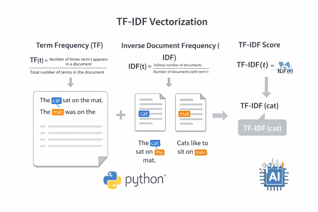
TF-IDF (Term Frequency–Inverse Document Frequency) is a classic weighting scheme that answers a simple question: how important is this word to this particular document, relative to how common it is across all documents?
A word like “the” appears everywhere, so its IDF score is near zero — it carries no discriminative power. But a word like “refund” that appears 5 times in one support ticket but rarely elsewhere gets a high TF-IDF score, signaling importance.
from sklearn.feature_extraction.text import TfidfVectorizer
from sklearn.model_selection import train_test_split

X = df["processed"].to_list()
y = df["label"].to_list()

X_train, X_test, y_train, y_test = train_test_split(
    X, y, test_size=0.2, random_state=42, stratify=y
)

vectorizer = TfidfVectorizer(
    max_features=15000,   # top 15k terms by TF-IDF score
    ngram_range=(1, 2),   # include bigrams ("credit card", "not working")
    sublinear_tf=True     # apply log normalization to term frequencies
)

X_train_tfidf = vectorizer.fit_transform(X_train)
X_test_tfidf  = vectorizer.transform(X_test)
TF-IDF is one of the most popular text vectorization techniques. Learn more in this tutorial on TF-IDF in Python.
Modern: Sentence Embeddings
TF-IDF treats every word as independent. It has no concept of synonyms, context, or meaning. “The app crashed” and “The application stopped working” would look completely different to TF-IDF, despite meaning the same thing.
Sentence embeddings — produced by models like sentence-transformers/all-MiniLM-L6-v2 — encode each sentence as a dense 384-dimensional vector where semantically similar sentences are geometrically close together. This contextual awareness is what makes transformer-based approaches so powerful.
from sentence_transformers import SentenceTransformer

# Load a compact but powerful sentence encoder
encoder = SentenceTransformer("all-MiniLM-L6-v2")

# Encode — returns numpy arrays of shape (n_samples, 384)
X_train_emb = encoder.encode(X_train, batch_size=64, show_progress_bar=True)
X_test_emb = encoder.encode(X_test, batch_size=64, show_progress_bar=True)| Method | Encoding Speed | Contextual? | Best For |
|---|---|---|---|
| TF-IDF | ⚡ Very fast | ❌ No | Baselines, simple tasks |
| Word2Vec / GloVe | ⚡ Fast | Partially | Word-level similarity |
| Sentence Transformers | 🔶 Moderate | ✅ Yes | Semantic search, few-shot |
| Fine-tuned BERT | 🔴 Slower | ✅ Full | High-accuracy production |
06Step 4: Building Models for Text Classification in Python — Two Paths
This is where the actual model training happens. We’ll build both paths so you can compare them directly on the same dataset.
Path A: The Fast Baseline — Logistic Regression
Don’t be fooled by the simplicity of Logistic Regression. With good TF-IDF features and enough data, it routinely achieves 85–92% accuracy on short text classification tasks. The scikit-learn Pipeline API makes it clean to build, tune, and deploy:
from sklearn.pipeline import Pipeline
from sklearn.linear_model import LogisticRegression
from sklearn.feature_extraction.text import TfidfVectorizer

# Build the pipeline: vectorize → classify in one object
lr_pipeline = Pipeline([
    ('tfidf', TfidfVectorizer(
        max_features=15000,
        ngram_range=(1, 2),
        sublinear_tf=True
    )),
    ('clf', LogisticRegression(
        C=5.0,          # regularization strength
        max_iter=1000,
        class_weight='balanced',  # handles class imbalance
        solver='lbfgs',
        n_jobs=-1       # use all CPU cores
    ))
])

# Train on raw text — the pipeline handles vectorization
lr_pipeline.fit(X_train, y_train)
lr_preds = lr_pipeline.predict(X_test)

print(f"Logistic Regression Accuracy: {lr_pipeline.score(X_test, y_test):.4f}")
🚀
Pipelines are production-ready
A scikit-learn Pipeline can be serialized with joblib.dump() and loaded back as a single object — vectorizer and model together. This prevents the infamous “train-test skew” bug where you apply different preprocessing at inference time.
Path B: The Powerhouse — DistilBERT Fine-tuning
Fine-tuning a pre-trained transformer is now genuinely accessible to any developer with a modern laptop. DistilBERT is a distilled version of BERT that retains 97% of its performance at 40% the size and 60% faster inference. The Hugging Face Trainer API handles the training loop, gradient accumulation, and evaluation for you:
from transformers import (
    AutoTokenizer, AutoModelForSequenceClassification,
    TrainingArguments, Trainer
)
from datasets import Dataset
import numpy as np

MODEL_NAME = "distilbert-base-uncased"
NUM_LABELS = len(set(y_train))

# Step 1: Load tokenizer and model
tokenizer = AutoTokenizer.from_pretrained(MODEL_NAME)
model = AutoModelForSequenceClassification.from_pretrained(
    MODEL_NAME, num_labels=NUM_LABELS
)

# Step 2: Tokenize the dataset
def tokenize_batch(batch):
    return tokenizer(
        batch["text"],
        padding="max_length",
        truncation=True,
        max_length=128
    )

train_hf = Dataset.from_dict({"text": X_train, "label": y_train})
test_hf  = Dataset.from_dict({"text": X_test,  "label": y_test})

train_tok = train_hf.map(tokenize_batch, batched=True)
test_tok  = test_hf.map(tokenize_batch,  batched=True)

# Step 3: Define training arguments
training_args = TrainingArguments(
    output_dir="./distilbert-support-classifier",
    num_train_epochs=3,
    per_device_train_batch_size=16,
    per_device_eval_batch_size=32,
    warmup_steps=100,
    weight_decay=0.01,
    evaluation_strategy="epoch",
    save_strategy="epoch",
    load_best_model_at_end=True,
    logging_dir="./logs",
)

# Step 4: Compute metrics function
def compute_metrics(eval_pred):
    logits, labels = eval_pred
    preds = np.argmax(logits, axis=-1)
    accuracy = (preds == labels).mean()
    return {"accuracy": accuracy}

# Step 5: Train!
trainer = Trainer(
    model=model,
    args=training_args,
    train_dataset=train_tok,
    eval_dataset=test_tok,
    compute_metrics=compute_metrics,
)

trainer.train()
With 3 epochs on a modern laptop CPU, expect training to take 15–30 minutes. On a GPU (even a free Colab T4), it drops to under 5 minutes. The resulting model will typically achieve 90–96% accuracy on well-curated text classification datasets — a significant improvement over the TF-IDF baseline for complex, nuanced language.
07Step 5: Evaluation & Interpreting Results
Accuracy is seductive, but it can be deeply misleading — especially on imbalanced datasets. A model that always predicts the majority class can achieve 90% accuracy while being completely useless. We need richer metrics.
Beyond Accuracy: Precision, Recall, and F1
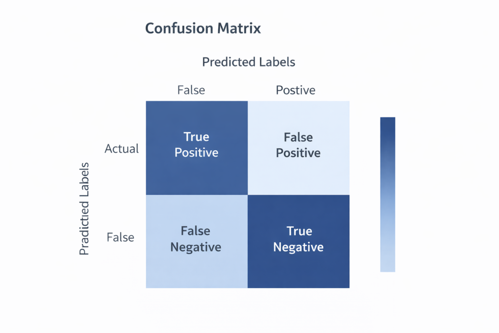
The Three Metrics That Matter
- Precision — of all the tickets I labeled “Billing,” how many actually were? (Measures false positives)
- Recall — of all the actual Billing tickets, how many did I catch? (Measures false negatives)
- F1-Score — the harmonic mean of precision and recall. The go-to metric when class balance is imperfect.
from sklearn.metrics import classification_report, confusion_matrix
import seaborn as sns
import matplotlib.pyplot as plt

# Full classification report
print(classification_report(y_test, lr_preds, digits=4))

# Confusion Matrix visualization
cm = confusion_matrix(y_test, lr_preds)
plt.figure(figsize=(10, 8))
sns.heatmap(
    cm,
    annot=True,
    fmt="d",
    cmap="Blues",
    xticklabels=sorted(set(y_test)),
    yticklabels=sorted(set(y_test))
)
plt.ylabel("True Label")
plt.xlabel("Predicted Label")
plt.title("Confusion Matrix — Logistic Regression")
plt.tight_layout()
plt.show()
The “Human Test”: Running Custom Queries
After looking at metrics, run a few handcrafted examples. This is the fastest way to spot behavioral quirks that aggregate metrics can hide:
test_queries = [
    "My credit card was charged twice for the same order",
    "The app keeps crashing when I open it on my phone",
    "My package has been stuck in transit for 10 days",
    "I can't log in, it says my password is wrong",
]

predictions = lr_pipeline.predict(test_queries)

for query, pred in zip(test_queries, predictions):
    print(f"Query: '{query[:50]}...'")
    print(f"  → Predicted Category: {pred}\n")
🎁Bonus: Zero-Shot Classification
What if you need to classify text into categories you never trained on? What if your requirements change tomorrow and you need to add a new label without retraining? Zero-shot classification makes this possible.
Large language models trained on massive text corpora develop such a strong understanding of language that they can classify text into arbitrary labels — provided you describe those labels in plain English. No training data required.
from transformers import pipeline

# Load a zero-shot classifier (uses facebook/bart-large-mnli under the hood)
zero_shot = pipeline("zero-shot-classification")

result = zero_shot(
    "The delivery arrived but the item was completely broken",
    candidate_labels=["billing issue", "damaged product", "account problem", "shipping delay"]
)

print(result["labels"][0])    # → "damaged product"
print(result["scores"][0])   # → 0.9721 (confidence)
Three lines, zero training data, and the model correctly identifies “damaged product” with 97% confidence. Zero-shot is not always as accurate as a fine-tuned model — but for prototyping, dynamic category sets, or cases with limited labeled data, it’s a remarkably powerful tool to have in your arsenal.
✨
When to use Zero-Shot
Zero-shot works best when your label names are descriptive and unambiguous. “Billing dispute” will outperform a cryptic label like “Category 3.” The model reads the label as a natural language phrase, so write it like one.
09Conclusion & Best Practices
When to Use What
| Situation | Recommended Approach | Why |
|---|---|---|
| Quick prototype, labeled data available | TF-IDF + Logistic Regression | Trains in seconds, easy to debug |
| High accuracy requirements, plenty of data | Fine-tuned DistilBERT | Best F1, handles nuance |
| No labeled data, flexible categories | Zero-Shot Classification | No training required |
| Semantic search + classification hybrid | Sentence Transformers + kNN | Embedding-based similarity |
| Edge deployment, mobile, IoT | Quantized ONNX model | Tiny footprint, fast inference |
Scalability in Production
Once your model performs well in notebook experiments, production brings new challenges. A few principles for 2026:
- Model Quantization: Convert your fine-tuned model to INT8 using
optimumor ONNX Runtime. This typically cuts model size by 75% and doubles inference speed with negligible accuracy loss. - Batching at Inference: Never call your model one sample at a time in production. Batch 32–64 requests together for GPU-efficient inference.
- On-Device NLP: Libraries like
llama.cppandMLC-LLMnow make it feasible to run small classifiers entirely on mobile hardware — zero data leaves the device, zero API costs, zero latency. - Data Drift Monitoring: Your model was trained on yesterday’s language. Set up periodic evaluation on fresh labeled samples to catch when accuracy starts to degrade.
Keep Experimenting
The field moves fast. What is “state of the art” today will be the new baseline in 18 months. The engineers who succeed are not the ones who memorize architectures — they’re the ones who understand the fundamentals well enough to adapt. You now have those fundamentals.
You’ve built a preprocessing pipeline with spaCy, trained a production-quality baseline with scikit-learn, fine-tuned a transformer with Hugging Face, and unlocked zero-shot classification for free-form category discovery. That’s a genuine, practical NLP toolkit.
The best next step is to take a real problem from your own work or life, gather some labeled data, and apply these techniques to something you actually care about. That hands-on repetition is what transforms tutorial knowledge into deep expertise.
📚
What to Explore Next
Named Entity Recognition (NER) with spaCy · Multi-label classification · Active Learning for efficient data labeling · Retrieval-Augmented Classification · LLM-based few-shot classifiers via the OpenAI or Anthropic APIs.
Another important NLP task is Named Entity Recognition in Python, which extracts entities such as people, locations, and organizations from text.
Frequently Asked Questions (FAQ)
What is text classification in Python?
Text classification in Python is the process of automatically assigning predefined categories to text using machine learning or deep learning models. Python libraries such as scikit-learn, spaCy, and Hugging Face Transformers make it easy to build text classifiers for tasks like spam detection, sentiment analysis, topic categorization, and support ticket routing.
Which algorithms are commonly used for text classification?
Several algorithms can be used for text classification depending on the complexity of the problem.
Common algorithms include:
Naive Bayes – fast and effective for simple text classification tasks
Logistic Regression – strong baseline model for TF-IDF features
Support Vector Machines (SVM) – good for high-dimensional text data
BERT / DistilBERT – deep learning models that understand context and semantics
For many beginner projects, TF-IDF with Logistic Regression is a great starting point.
What is the difference between sentiment analysis and text classification?
Sentiment analysis is actually a type of text classification.
The difference is:
Task Description
Text Classification Assigns text to predefined categories
Sentiment Analysis Classifies text based on sentiment (positive, negative, neutral)
For example:
Sentence: “The app crashes every time I open it.”
Text classification → Technical Issue
Sentiment analysis → Negative
Do I need deep learning for text classification?
No. Many real-world text classification systems still use traditional machine learning models like Logistic Regression or Naive Bayes.
These models can achieve 85–92% accuracy with techniques such as TF-IDF vectorization.
Deep learning models like BERT are useful when:
language is complex
context matters heavily
very high accuracy is required
What libraries are used for text classification in Python?
Popular Python libraries for text classification include:
scikit-learn – traditional machine learning models
spaCy – text preprocessing and NLP pipelines
Hugging Face Transformers – modern deep learning NLP models
NLTK – classic NLP toolkit for text processing
These tools allow developers to build powerful NLP applications with relatively small amounts of code.
What are real-world applications of text classification?
Text classification is widely used in modern AI systems.
Common applications include:
Email spam detection
Sentiment analysis for product reviews
Customer support ticket routing
Topic classification for news articles
Intent detection in chatbots
Content moderation on social media platforms
Because large amounts of digital text are created every day, text classification has become one of the most important tasks in Natural Language Processing (NLP).